Modular Framework for Uncertainty Prediction in Autonomous Vehicle Motion Forecasting within Complex Traffic Scenarios

Abstract

We propose a modular modeling framework designed to enhance the capture and validation of uncertainty in autonomous vehicle (AV) trajectory prediction. Departing from traditional deterministic methods, our approach employs a flexible, end-to-end differentiable probabilistic encoder-decoder architecture. This modular design allows the encoder and decoder to be trained independently, enabling seamless adaptation to diverse traffic scenarios without retraining the entire system. Our key contributions include: (1) a probabilistic heatmap predictor that generates context-aware occupancy grids for dynamic forecasting, (2) a modular training approach that supports independent component training and flexible adaptation, and (3) a structured validation scheme leveraging uncertainty metrics to evaluate robustness under high-risk conditions. To highlight the benefits of our framework, we benchmark it against an end-to-end baseline, demonstrating faster convergence, improved stability, and flexibility. Experimental results validate these advantages, showcasing the capacity of the framework to efficiently handle complex scenarios while ensuring reliable predictions and robust uncertainty representation. This modular design offers Asignificant practical utility and scalability for real-world autonomous driving applications.

Keywords Modular Framework, Generative Model, Probabilistic Motion Prediction, Autonomous Vehicles

1 Introduction

Autonomous vehicle (AV) driving has emerged as a transformative technology with the potential to revolutionize transportation systems. Previous research presents the potential of improving the fuel efficiency and throughput of overall traffic flow via a small penetration rate of AV[1, 2, 3]. A critical component of this paradigm is trajectory prediction, which involves forecasting the future positions of vehicles and other road users. Accurate predictions are essential for ensuring safety and operational efficiency in dynamic traffic environments. However, inherent uncertainties in road conditions, driver behaviors, and sensor inaccuracies pose significant challenges to conventional trajectory prediction models.

Existing approaches in AV trajectory prediction typically rely on deterministic models, which assume a single, most likely outcome for vehicle trajectories [4]. While these methods are computationally efficient, they fail to capture the uncertainty inherent in real-world driving scenarios. Probabilistic models have been introduced to address this limitation, offering predictions in the form of distributions or likelihoods over future trajectories [5]. Weng et al. [6] proposed PARA-Drive, a modular and differentiable framework for trajectory prediction in autonomous driving, enabling interpretable multi-agent interaction modeling through occupancy prediction and action refinement. Despite these advancements, most models are limited by their monolithic training frameworks, which often compromise flexibility and adaptability across diverse traffic conditions.

Several studies have identified limitations in conventional trajectory prediction systems, particularly in representing uncertainty. Probabilistic models, such as Gaussian Mixture Models (GMMs) and Variational Autoencoders (VAEs), have been employed to forecast multiple plausible future trajectories  [5, 7, 8]. However, these approaches face challenges in dynamic traffic environments with unpredictable agent interactions  [9, 10].

GMMs assume that data can be represented as a mixture of Gaussian distributions, which may not capture the complexity of real-world driving scenarios. This can lead to oversimplified predictions, especially in situations involving abrupt lane changes or unconventional maneuvers. For example, Wiederer et al. [9] noted that GMMs might not effectively model the intricacies of dynamic traffic environments.

VAEs provide a framework for learning variational models using neural networks and can incorporate various distributional assumptions, including GMMs, within their latent spaces. The flexibility of VAEs depends on the choice of prior and variational distributions. For instance, Neumeier et al.  [7] introduced a VAE-based vehicle trajectory prediction model with an interpretable latent space, demonstrating the adaptability of VAEs in modeling complex behaviors. However, selecting the appropriate number of components in GMMs remains a challenge. An incorrect choice can result in models that either fail to capture all relevant behaviors or include redundant components, complicating the prediction process. Salzmann et al.  [11] addressed this by employing a VAE with a GMM before modeling multimodal human trajectories, highlighting the importance of choosing suitable model structures.

While probabilistic models like GMMs and VAEs offer frameworks for capturing uncertainties in trajectory prediction, their effectiveness is contingent upon appropriate modeling choices and assumptions. Careful selection of model parameters and structures is essential to represent the complexities of real-world driving scenarios accurately.

Another notable challenge in existing trajectory prediction methods is the flexibility of the architectures in tackling different tasks or transferring pretraining to other scenarios. Many state-of-the-art models rely on monolithic encoder-decoder frameworks trained end-to-end to maximize overall performance. While these frameworks can deliver high predictive accuracy, their lack of modularity makes it difficult to adapt individual components to task-specific requirements. For example, in situations where distinct prediction objectives such as occupancy heatmaps and precise trajectory forecasts are needed, jointly trained models cannot effectively optimize for each task independently [12]. This limitation reduces the adaptability of these models when deployed in new environments or when required to incorporate additional data modalities, such as high-definition maps or updated traffic behavior models. While retraining a monolithic model might be feasible in certain offline settings, such an approach becomes impractical in scenarios requiring frequent updates or real-time adaptation. For instance, autonomous vehicle systems operating in diverse geographical regions must continuously integrate new data reflecting local traffic dynamics, infrastructure changes, or weather variations. In such cases, retraining a monolithic model incurs repeated computational costs and delays in deployment, which can be particularly detrimental for time-sensitive applications.

Moreover, certain edge-case scenarios necessitate on-board or online model adaptation. For example, in rapidly evolving traffic conditions, such as during natural disasters or unexpected road closures, retraining the entire model offline is infeasible due to time constraints. Modular frameworks, by contrast, allow selective retraining of specific components, such as decoders for occupancy heatmaps, without requiring end-to-end retraining. This adaptability not only reduces computational overhead but also facilitates rapid updates to maintain performance parity or even improve over monolithic models.

The semantic representation method of features is also an important design dimension that affects the learning-based control systems[6, 13]. Besides static prediction of deterministic trajectory, heatmap-based occupancy predictors have emerged as a promising solution to capture the probabilistic distribution of future positions [14]. However, these models frequently fail to integrate contextual information from the surrounding traffic environment effectively. This limitation results in predictions that may be spatially coherent but contextually irrelevant, such as assigning high probabilities to non-drivable areas or neglecting critical cues from the trajectories of other road users [15]. Furthermore, the temporal resolution of these predictors often does not align well with the dynamic nature of real-time traffic, leading to delayed or overly smoothed predictions that hinder the ability to respond to rapidly evolving scenarios [16].

To address these challenges, this paper introduces a modular framework for autonomous vehicle trajectory prediction, with a focus on probabilistic occupancy heatmap generation. The proposed methodology builds on the limitations of existing models by:

• Introducing a Modular Training Approach: This framework decouples the training of encoders and decoders, allowing for independent optimization and greater adaptability to task-specific requirements.

• Developing a Heatmap Predictor: By generating probabilistic occupancy grids, the model provides context-sensitive uncertainty representation, enhancing AV systems’ ability to anticipate and mitigate potential collisions.

• Designing a Robust Validation Scheme: The framework evaluates performance using uncertainty-aware metrics, demonstrating its efficacy across diverse traffic scenarios.

Experimental evaluations using real-world (Argoverse 2) and simulated datasets (SUMO) demonstrate that the modular framework significantly improves spatial alignment and predictive accuracy. The model achieves state-of-the-art performance in uncertainty representation, validated through comparisons with baseline architectures.

Figure 1: Proposed Modular Framework for Autonomous Vehicle Prediction Tasks: The framework comprises an upstream perception layer, a general encoder, and task-specific decoders. The perception layer collects data from onboard sensors, V2X, and other sources, which the encoder processes into a latent matrix capturing spatial and temporal information. This matrix is shared across decoders, enabling specialized tasks like occupancy and trajectory prediction. The modular design allows independent optimization of the encoder and decoders, enhancing adaptability and supporting task-specific fine-tuning while maintaining end-to-end differentiability. This paper emphasizes the encoder and decoder levels, focusing on uncertainty modeling through occupancy heatmap generation.

2 Methodology

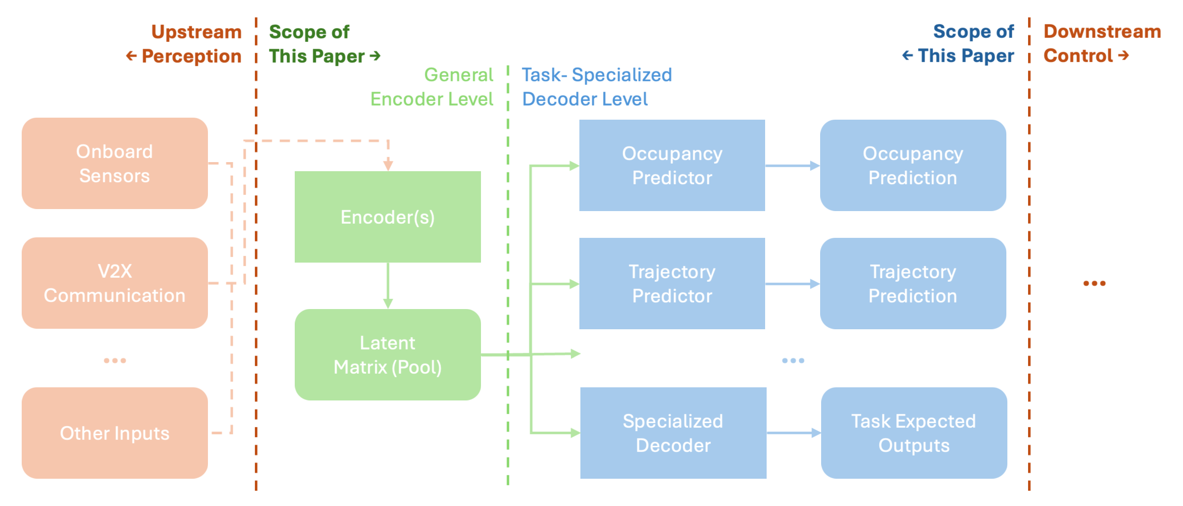
In this section, we introduce our end-to-end differentiable modular framework designed for autonomous vehicle (AV) prediction tasks. This flexible architecture, illustrated in Fig. 1, consists of a general encoder that processes upstream perception data and multiple task-specialized decoders that cater to distinct prediction needs. A key novelty of our approach is the independent training of encoder and decoder components, which allows efficient adaptation to new tasks without reconfiguring the entire model. To illustrate the power of this modular framework, we focus on probabilistic occupancy heatmap prediction, a task particularly well-suited for capturing spatial uncertainty in dynamic traffic scenarios.

Heatmaps provide a probabilistic view of future vehicle positions by discretizing the spatial environment into grid cells, each representing the likelihood of occupancy at specific future times. This method allows us to quantify uncertainty in vehicle trajectories and enables the AV system to anticipate potential collisions and adapt to varying traffic conditions. Figures 3 and 4 detail the encoder-decoder structure and the modular training methodology used in our heatmap prediction framework.

2.1 General End-to-End Differentiable Architecture

Our proposed architecture is a modular, end-to-end differentiable framework designed to accommodate diverse prediction tasks required for autonomous vehicle (AV) control, as shown in Figure 1. The framework begins at the encoder level, where incoming data from perception systems (e.g., onboard sensors and V2X communication) and location-centered roadway information are processed to produce a shared latent representation. This latent representation, structured as a latent matrix or feature pool, captures spatial and temporal dependencies essential for downstream prediction tasks.

The encoder level operates as a general feature extractor, transforming raw input data into high-dimensional embeddings that encapsulate relevant environmental and contextual information. This latent matrix then serves as a shared resource, providing a common feature space for multiple task-specific decoders, each tailored to a unique prediction objective, such as occupancy prediction, trajectory forecasting, or other specialized tasks.

At the decoder level, the architecture supports a range of task-specialized decoders, each independently optimized for its respective prediction task. This setup allows for flexible and modular adaptation, where new decoders can be integrated or existing ones replaced without retraining the entire system. For example, distinct decoders could be tailored for predicting trajectories of specific agent types such as pedestrians, bicyclists, and motorized vehicles, each of which exhibits unique motion patterns and interaction dynamics. Additionally, task-specialized decoders may address scenarios requiring occupancy heatmaps for high-risk areas like intersections or trajectory forecasts for highway merging zones. These decoders leverage the shared latent representation generated by the encoder, ensuring the contextual richness of predictions while adapting to the specific requirements of each task.

The primary advantage of this modular design is its ability to independently train encoder and decoder components, which enhances flexibility and adaptability. By allowing separate optimization of each module, the framework maintains high adaptability to new tasks and scenarios while preserving end-to-end differentiability, facilitating efficient fine-tuning when required. In this paper, we demonstrate this modular framework through a focus on probabilistic occupancy heatmap prediction, which serves as a case study to showcase the model’s ability to capture uncertainty in dynamic traffic environments.

Figure 2: Illustration of the elements in the traffic scenario: traffic (including AV), target vehicle and map.

2.2 Heatmap Prediction Framework

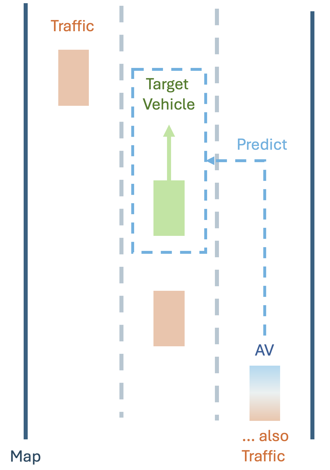
Figure 2 provides an illustration of the elements in the traffic scenario of interest. The target vehicle (green) is the subject of prediction, and the goal is to generate a probabilistic heatmap predicting the future spatial positions that are likely to be occupied by this vehicle. Surrounding traffic (orange), including the autonomous vehicle (blue, labeled as "AV"), contributes contextual information, such as trajectories and interactions, that influence the target vehicle’s motion. The map data includes lane boundaries and road structure, which provide static environmental context. This prediction task enables the AV to anticipate the target vehicle’s future positions, helping it adapt its driving strategy to avoid potential collisions, maintain safe distances, or make informed decisions about lane changes and merging in dynamic traffic environments.

To implement the proposed architecture with a specific prediction task, we introduce the realtime probabilistic occupancy heatmap prediction using the map and trajectory data of target and traffic vehicles. Let $H_{t_{k}}$ represent the heatmap at future time $t_{k}$, where each grid cell in $H_{t_{k}}$ denotes the occupancy probability of the target vehicle. At any given time $t_{0}$, the objective is to predict these heatmaps over $K$ future time steps to anticipate potential occupancy of the target vehicle. Formally, we aim to compute the heatmap of a target vehicle (i.e., predict the motion for each of the vehicles surrounding the AV):

$$H_{t_{k}}=F(\mathbf{T}_{\text{target}},\mathbf{T}_{\text{traffic}},\mathbf{M};\theta_{e},\theta_{d}),$$ (1)

where $F$ denotes the end-to-end differentiable function with parameters $\theta_{e}$ for the encoder and $\theta_{d}$ for the decoder. The inputs to this function are:

• $\mathbf{T}_{\text{target}}$: Past trajectory data of the target vehicle, represented as $\mathbf{T}_{\text{target}}=\{\mathbf{x}_{t_{i}}\}_{i=-I}^{0}$, where $\mathbf{x}_{t_{i}}\in\mathbb{R}^{2}$ denotes position at time $t_{i}$.

• $\mathbf{T}_{\text{traffic}}$: Trajectories of surrounding traffic objects, $\mathbf{T}_{\text{traffic}}=\{\mathbf{T}_{n}\}_{n=1}^{N}$, with each $\mathbf{T}_{n}=\{\mathbf{x}_{n,t_{i}}\}_{i=-I}^{0}$ for object $n$.

• $\mathbf{M}$: Vectorized map data capturing static road elements, such as boundaries and lane markings.

The architecture allows the encoder to process these inputs into a shared latent representation, which is then fed into multiple decoders for specific tasks, such as occupancy and trajectory prediction. This modular setup enhances flexibility, allowing each encoder-decoder pair to be trained independently for specific prediction tasks.

Focusing on heatmap prediction provides a means to capture the uncertainty inherent in dynamic traffic environments around AV. Heatmaps are generated as probabilistic occupancy grids, explicitly predicting the likelihood of vehicle presence in specific grid cells over time. These grids represent the occupancy of surrounding vehicles within the scene. By predicting these probabilistic distributions rather than deterministic trajectories, the framework accommodates the unpredictability of surrounding vehicles, providing AVs with a robust tool to anticipate and react to potential risks.

Figure 3: Attention-Based Encoder for Modular Feature Extraction in Autonomous Vehicle Prediction: in the heatmap prediction case, the encoder processes multiple input streams, including traffic data, map information, and target trajectory, to generate a shared latent representation that captures spatial and temporal dependencies. Each input type is processed independently through self-attention heads, such as the traffic and map heads, which extract relevant features into an environment latent matrix. The cross-attention mechanism further refines this matrix by integrating information across the input sources, producing a unified latent matrix (pool) that serves as a contextual embedding for downstream prediction tasks. During encoder training, a pre-trained decoder with frozen parameters is attached, allowing the encoder to adaptively learn features that align with the input requirements of decoders.

Figure 4: Decoder Training Process with Generative Adversarial Network (GAN) for Occupancy Prediction: the encoder is detached to allow independent training of the task-specialized decoder. The decoder utilizes a GAN architecture, where the generator (occupancy predictor or ’heatmapper’) receives input noise and produces probabilistic occupancy heatmaps, representing the likelihood of vehicle occupancy across a spatial grid. The GAN discriminator assesses the realism of these generated heatmaps by distinguishing them from real samples, with an additional ’judge’ component evaluating the output quality based on task-specific metrics.

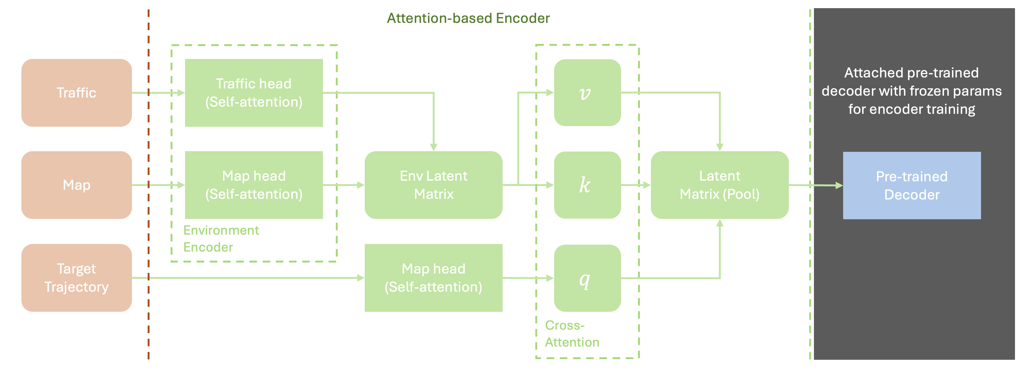
2.2.1 Encoder: Transformer-based Context Extractor

The encoder, parameterized by $\theta_{e}$, is responsible for extracting meaningful features from the input data $\mathbf{T}_{\text{target}}$, $\mathbf{T}_{\text{traffic}}$, and $\mathbf{M}$, producing a latent matrix $\mathbf{Z}\in\mathbb{R}^{d_{z}}$ that captures the spatial and temporal context relevant for prediction. The encoder employs self-attention and cross-attention mechanisms to achieve this.

Each input component is first encoded individually. The target vehicle’s trajectory, surrounding traffic, and map data are transformed into embeddings using self-attention (SA) layers. Let $\mathbf{E}_{\text{target}}$, $\mathbf{E}_{\text{traffic}}$, and $\mathbf{E}_{\text{map}}$ represent these encoded inputs:

$$\mathbf{E}_{\text{target}} =\text{SA}(\mathbf{T}_{\text{target}})\in\mathbb{R}^{d_{z}},$$ (2)

$$\mathbf{E}_{\text{traffic}} =\{\text{SA}(\mathbf{T}_{n})\}_{n=1}^{N}\in\mathbb{R}^{N\times d_{z}},$$ (3)

$$\mathbf{E}_{\text{map}} =\text{SA}(\mathbf{M})\in\mathbb{R}^{d_{z}}.$$ (4)

The self-attention layers $\text{SA}(\cdot)$ map each input type into an embedding space of dimension $d_{z}$. These embeddings are then processed through a cross-attention mechanism to dynamically emphasize contextually relevant features. Let $\mathbf{Q}$, $\mathbf{K}$, and $\mathbf{V}$ represent the query, key, and value matrices, computed as follows:

$$\mathbf{Q} =\text{Linear}(\mathbf{E}_{\text{target}}),$$ (5)

$$\mathbf{K} =\text{Linear}(\mathbf{E}_{\text{traffic}}\oplus\mathbf{E}_{\text{map}}),$$ (6)

$$\mathbf{V} =\text{Linear}(\mathbf{E}_{\text{traffic}}\oplus\mathbf{E}_{\text{map}}),$$ (7)

where $\oplus$ represents concatenation. The cross-attention output is computed as:

$$\text{Attention}(\mathbf{Q},\mathbf{K},\mathbf{V})=\text{softmax}\left(\frac{\mathbf{Q}\mathbf{K}^{\top}}{\sqrt{d_{k}}}\right)\mathbf{V},$$ (8)

producing the latent matrix $\mathbf{Z}$ that serves as a shared context for prediction tasks. This matrix encapsulates both the temporal sequence of vehicle trajectories and spatial environmental factors, providing a comprehensive representation for the decoder.

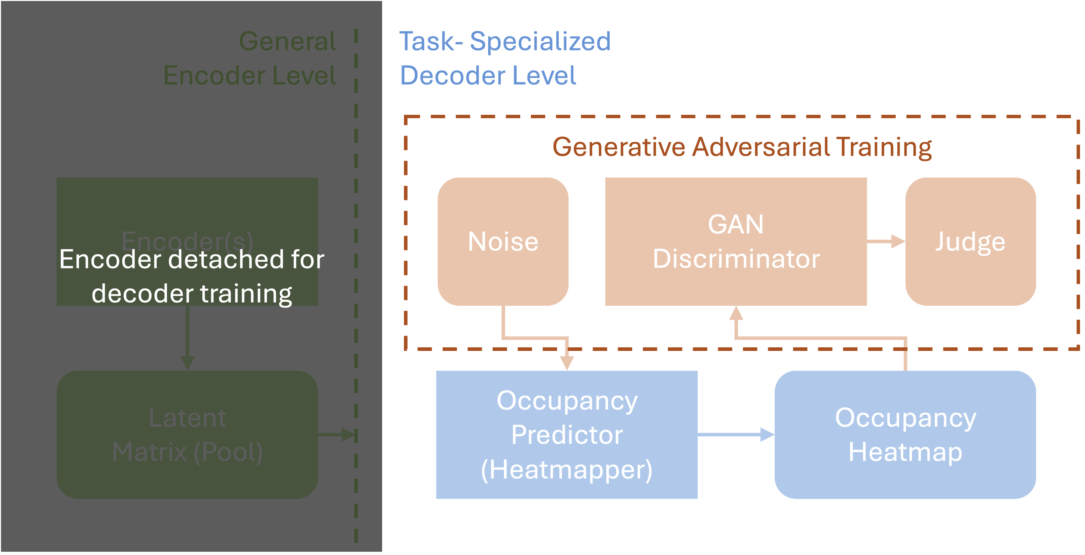
2.2.2 Decoder: GAN-based Occupancy Heatmap Generator

The GAN-based decoder, parameterized by $\theta_{d}$, translates the latent matrix $\mathbf{Z}$ into probabilistic occupancy heatmaps $\{H_{t_{k}}\}_{k=1}^{K}$, where each grid cell $(i,j)$ in $H_{t_{k}}$ holds the probability of vehicle occupancy at future time $t_{k}$. This probabilistic approach allows the model to represent uncertainty, as it predicts a range of potential future positions for each traffic participant. In this paper, the decoder is pre-trained in the GAN framework separately before being connected to an encoder. The specification of the training procedure will be elaborated in Section 2.3.

The generator $G$ in the GAN takes a latent vector $\mathbf{z}_{t_{k}}$ extracted from $\mathbf{Z}$ and generates a heatmap $H_{t_{k}}$:

$$H_{t_{k}}=G(\mathbf{z}_{t_{k}};\theta_{d}),$$ (9)

where $\mathbf{z}_{t_{k}}$ is contextually adapted to represent specific prediction requirements for time $t_{k}$. The probability of occupancy at each grid cell $(i,j)$ is defined as:

$$H_{t_{k}}(i,j)=\text{P}(\text{occupancy at grid cell }(i,j)\mid t_{k}).$$ (10)

The discriminator $D$ in the GAN is trained to distinguish between real and generated heatmaps, enforcing realism in $G$ outputs through an adversarial loss function:

$$\min_{G}\max_{D}V(D,G) =\mathbb{E}_{\mathbf{x}\sim p_{\text{data}}}[\log D(\mathbf{x})]$$ (11)

$$\quad+\mathbb{E}_{\mathbf{z}\sim p_{z}}[\log(1-D(G(\mathbf{z})))],$$

where $\mathbf{x}$ represents real heatmaps and $\mathbf{z}$ is sampled from the latent distribution $p_{z}$. This adversarial training ensures that generated heatmaps display plausible probabilistic occupancy distributions.

2.3 Modular Training Approach

Our modular approach separates encoder and decoder training into distinct phases, enhancing flexibility, stability, and task-specific adaptability.

Figure 5: Initial Heatmap Outputs Generated by the GAN Decoder Without Encoder Attached: These heatmaps are produced solely by the GAN decoder from noise inputs, without any predictive meaning at this stage.

2.3.1 Independent Decoder Training

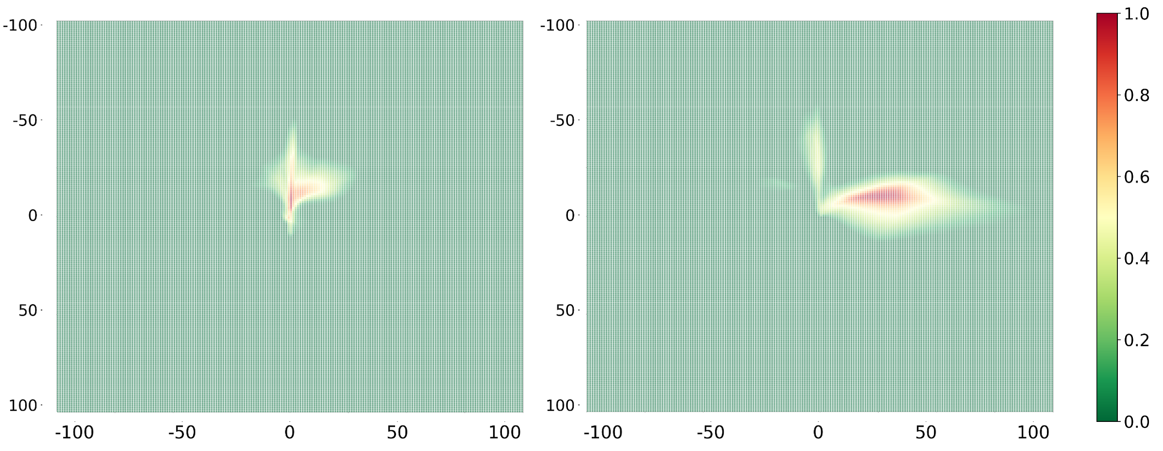
The decoder is first trained independently using the adversarial loss defined above. The resolution of the heatmap (i.e., the number of cells in each dimension) is a design parameter that balances granularity with computational efficiency. The heatmap dataset used for pre-training the generator is obtained through a simulation process. Specifically, the process begins by identifying specific locations along the road, referred to as "trigger points." These trigger points are selected to represent key areas of interest, such as intersections, merging zones, or straight road segments. For each trigger point, the trajectories of vehicles are recorded after they pass the designated location. These trajectories include detailed positional information over time, which is then used to construct probabilistic heatmaps. For every trigger point, we generate a sequence of $K$ occupancy heatmaps, where each heatmap corresponds to a specific future time frame within a predefined prediction horizon. These heatmaps represent the likelihood of vehicle presence in each grid cell, providing a temporal snapshot of the dynamic traffic environment around the trigger point. Figure 5 provides two samples of heatmaps generated from the noise. The goal of this initial decoder-only training phase is to enable the GAN generator to produce ’realistic-looking’ probabilistic occupancy heatmaps that emulate plausible spatial distributions. This phase ensures the ability to generate coherent heatmap structures, establishing a foundation for the next phase where the encoder will be trained to utilize the decoder effectively for generating meaningful, context-aware predictions.

2.3.2 Encoder Training with Fixed Decoder

Once the decoder is pre-trained, the encoder is trained with the weights of the decoder fixed. Using the ground truth of occupancy mapped by snapshots of the trajectory over time as the ground-truth heatmaps $\{H_{t_{k}}\}_{k=1}^{K}$, the encoder is optimized to produce latent representations that align with the pre-trained decoder output.

The encoder is trained using a cross-entropy loss, suitable for probabilistic prediction tasks:

$$L=-\frac{1}{C}\sum_{c=1}^{C}\left[y_{c}\log(\hat{y}_{c})+(1-y_{c})\log(1-\hat{y}_{c})\right],$$ (12)

where $C$ is the number of cells, $y_{c}$ is the ground-truth occupancy for cell $c$, and $\hat{y}_{c}$ is the predicted probability.

2.3.3 End-to-End Fine-Tuning

An optional fine-tuning phase jointly optimizes both encoder and decoder, further refining the model’s overall predictive capability:

$$\min_{\theta_{e},\theta_{d}}L(\mathbf{H},\hat{\mathbf{H}}),$$ (13)

where $\mathbf{H}$ and $\hat{\mathbf{H}}$ denote true and predicted heatmaps. This final stage preserves modularity while optimizing the interactions between $\theta_{e}$ and $\theta_{d}$.

3 Experiments and Results

This section describes the experimental setup, training procedure, and performance evaluation of the proposed modular framework for probabilistic occupancy heatmap generation. The goal is to assess the accuracy of the heatmaps, their spatial alignment with drivable areas, and the ability to capture uncertainties relevant to autonomous vehicle operations.

3.1 Experimental Setup

The proposed framework was evaluated using both real-world and simulated datasets:

• Real-World Data: The Argoverse 2 Motion Forecasting Dataset [17] provides trajectory data for various traffic agents across diverse urban environments. These annotations include positional information, lane geometries, and context-relevant metadata.

• Simulated Data: The SUMO (Simulation of Urban MObility) platform was utilized to create synthetic traffic scenarios. These simulations reconstructed real-world road layouts from six U.S. cities in the Argoverse dataset: Austin, (TX); Detroit (MI); Miami, (FL); Pittsburgh, (PA); Palo Alto, (CA); and Washington, D.C. SUMO’s capability to model diverse scenarios such as intersections, highways, and mixed traffic enabled the generation of rich occupancy heatmaps. For each scenario, we defined trigger points to capture vehicle trajectories and aggregated probabilistic heatmaps for $K$ future frames.

The combined dataset enabled the model to generalize across various traffic conditions, enhancing its practical utility.

3.2 Training Procedure

The training process was designed in multiple modular phases to ensure flexibility and adaptability.

3.2.1 Initial Decoder Training Using GAN

The decoder (Decoder 0) was initially trained using a Generative Adversarial Network (GAN) framework. The objective was to generate visually realistic heatmaps that represent potential vehicle occupancies.

The GAN setup involved:

• Generator ($G$): The decoder received noise vectors $\mathbf{z}\sim p_{z}$ as input and generated heatmaps $H_{t_{k}}$.

• Discriminator ($D$): Trained to distinguish between real heatmaps from the dataset ($H_{\text{real}}$) and generated heatmaps ($H_{\text{gen}}=G(\mathbf{z})$).

The adversarial loss was optimized as:

$$\begin{split}\min_{G}\max_{D}\mathcal{L}(D,G)=&\ \mathbb{E}_{H_{\text{real}}\sim p_{\text{data}}}[\log D(H_{\text{real}})]\\ &+\mathbb{E}_{\mathbf{z}\sim p_{z}}[\log(1-D(G(\mathbf{z})))].\end{split}$$ (14)

where $p_{\text{data}}$ is the true data distribution. After this phase, Decoder 0 generated heatmaps that appeared visually realistic but lacked meaningful alignment with drivable areas.

3.2.2 Encoder-Decoder Integration and Encoder Training

To enable task-specific prediction, the decoder was integrated with an encoder. The decoder parameters were frozen and the encoder was trained to output feature matrices that aligned with the input dimensions of the decoder.

The encoder is tasked with mapping the input data, $(\mathbf{T}_{\text{target}},\mathbf{T}_{\text{traffic}},\mathbf{M})$, which includes spatiotemporal context, into latent representations $\mathbf{Z}$ optimized for heatmap generation and to minimize the prediction loss indicated by equation (12):

$$\mathbf{Z}=f_{\theta_{e}}(\mathbf{T}_{\text{target}},\mathbf{T}_{\text{traffic}},\mathbf{M}),$$ (15)

where $f_{\theta_{e}}$ represents the encoder with parameters $\theta_{e}$.

Two encoder variants were trained:

• Encoder 0: Trained exclusively on Argoverse data.

• Encoder 1: Trained on both Argoverse and SUMO data to generalize across diverse scenarios.

3.2.3 Decoder Fine-Tuning

To address non-drivable area predictions, we fine-tuned the decoder with additional constraints:

• Filtered Dataset ($\mathcal{D}_{\text{filtered}}$): Samples that use pedestrian or bike as the target agent were excluded, ensuring that the training data focused solely on drivable regions.

• Drivable Area Penalty: A penalty term was added to the loss function:

  $$\mathcal{L}_{\text{penalty}}=\lambda\sum_{(i,j)\notin\text{Drivable}}H_{t_{k}}(i,j),$$ (16)

  where $\lambda$ is a penalty weight, and $(i,j)$ indexes grid cells outside the drivable area.

Two fine-tuned decoder variants were created:

• Decoder 1: Trained with $\mathcal{D}_{\text{filtered}}$.

• Decoder 2: Trained with $\mathcal{D}_{\text{filtered}}$ and $\mathcal{L}_{\text{penalty}}$.

(a) Encoder 0 + Decoder 0
(4.7902%)

(b) Encoder 0 + Decoder 1
(0.2163%)

(c) Encoder 0 + Decoder 2
(0.0247%)

(d) Encoder 1 + Decoder 0
(5.1839%)

(e) Encoder 1 + Decoder 1
(0.5471%)

(f) Encoder 1 + Decoder 2
(0.0658%)

Figure 6: Comparison of Heatmaps Generated by Various Encoder-Decoder Configurations. The figure illustrates occupancy heatmaps produced by combinations of different encoder and decoder configurations, wherein The percentage in brackets represents the proportion of total values of cells outside the drivable area. Figures (a) and (d) represent the outputs from Decoder 0 before fine-tuning, paired with Encoder 0 and Encoder 1, respectively. The second column, figures (b) and (e), shows the results after fine-tuning using Decoder 1, which was trained on a filtered dataset excluding non-drivable areas. The third column, figures (c) and (f), presents the outputs after fine-tuning with Decoder 2, which incorporated both filtered data and a drivable area penalty. Progressive improvements are observed across columns, with configurations involving Decoder 2 (figures c and f) exhibiting the most accurate spatial alignment and confinement of probabilities within drivable regions. These results emphasize the significance of fine-tuning in enhancing the realism and practical applicability of the generated heatmaps for autonomous vehicle systems.

3.3 Comparative Analysis of Heatmap Predictions

To validate the advantages of the proposed modular training approach, we compare it against a benchmark framework trained end-to-end without pretraining or fine-tuning. This benchmark shares the same architecture as Encoder 0 and Decoder 0 but does not leverage the modular design, pretraining or finetuning.

Figure 7 illustrates two training curves: the benchmark model and the modular framework. For a fair comparison, the training curve of the modular framework accounts for the decoder pretraining time by shifting its starting point on the time axis by an offset equivalent to the pretraining duration. This adjustment reflects the cumulative effort required for modular training.

The benchmark model demonstrates significantly slower convergence, requiring over 170% wall time on average to reach comparable validation loss levels achieved by the modular framework, including pretraining time. Additionally, the benchmark model exhibits high instability, failing to converge in 39% of experiments. This instability arises from the lack of modular pretraining, which hinders the ability to adapt efficiently to the task-specific prediction requirements.

Figure 7: Comparison of Learning Curves for Modular and End-to-End Training Approaches: The green-shaded region highlights the decoder pretraining phase for the modular framework, after which its training curve shifts to the right by the pretraining duration. The modularized approach exhibits faster convergence, lower variance, and greater stability compared to the end-to-end method, which suffers from slower convergence and higher instability.

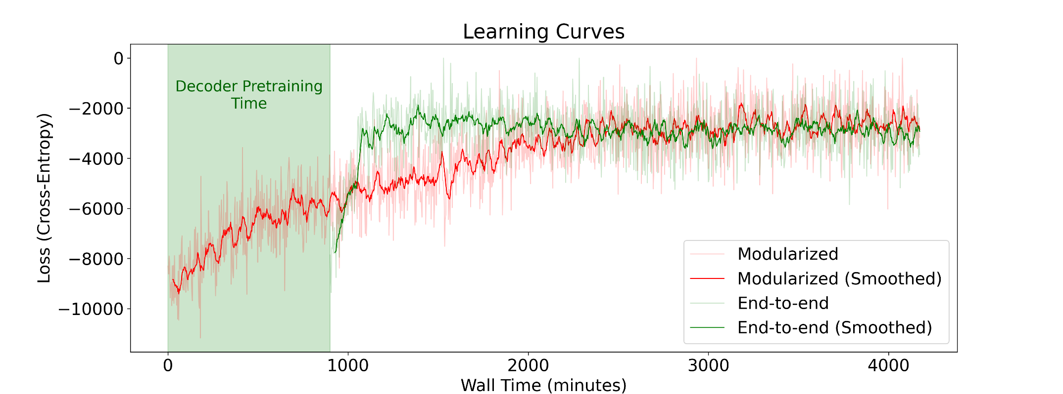
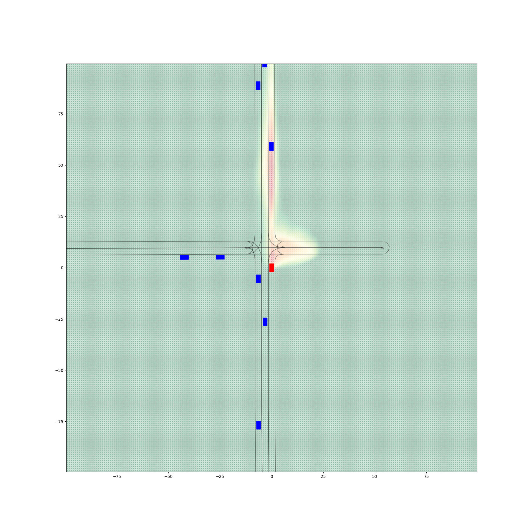
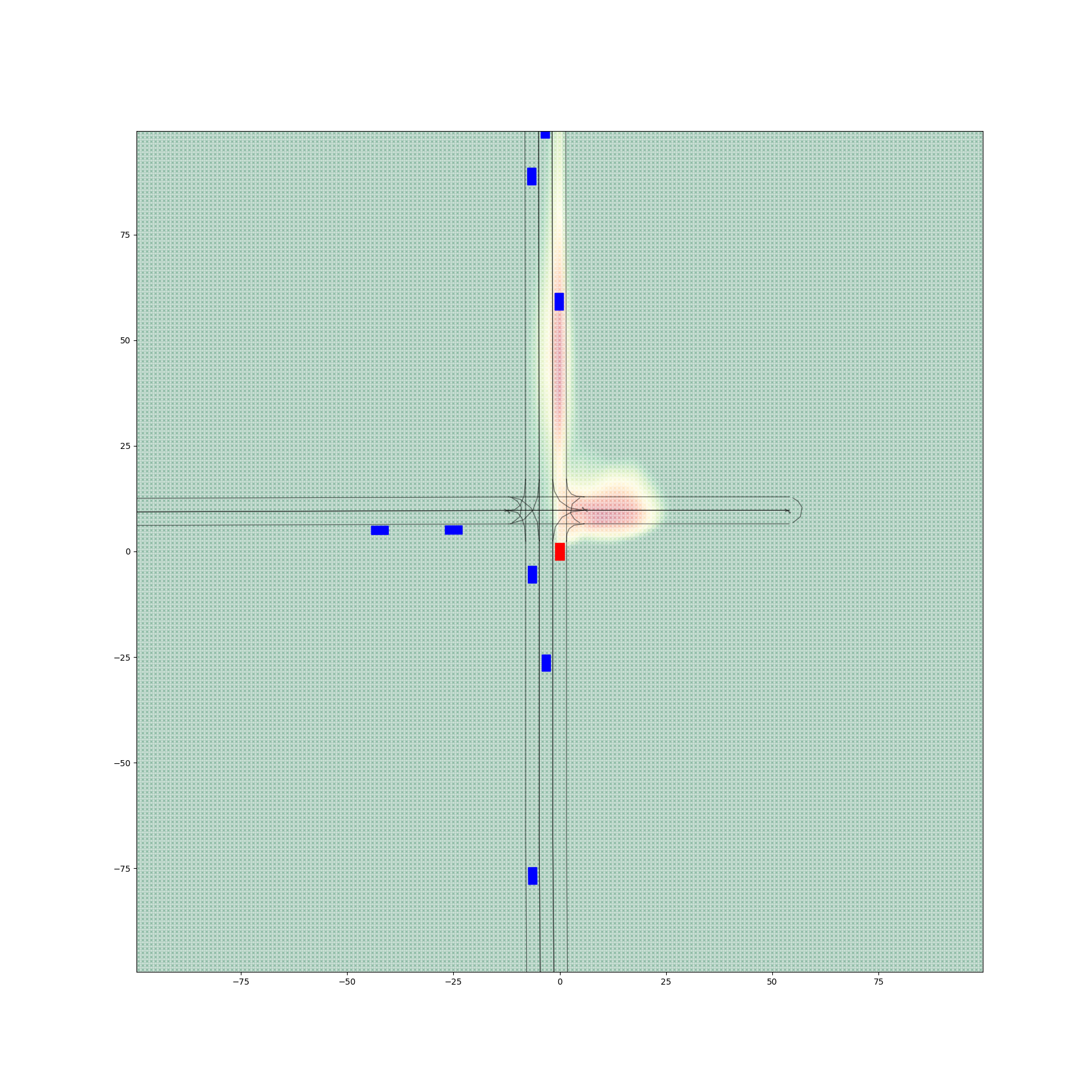
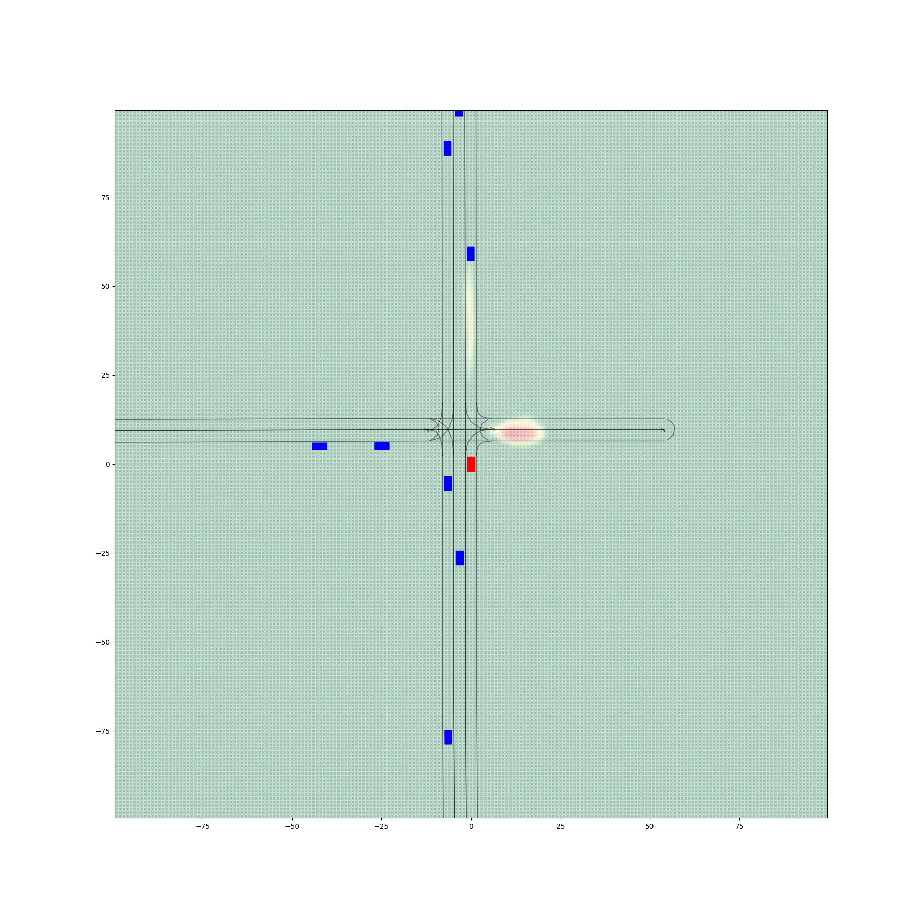
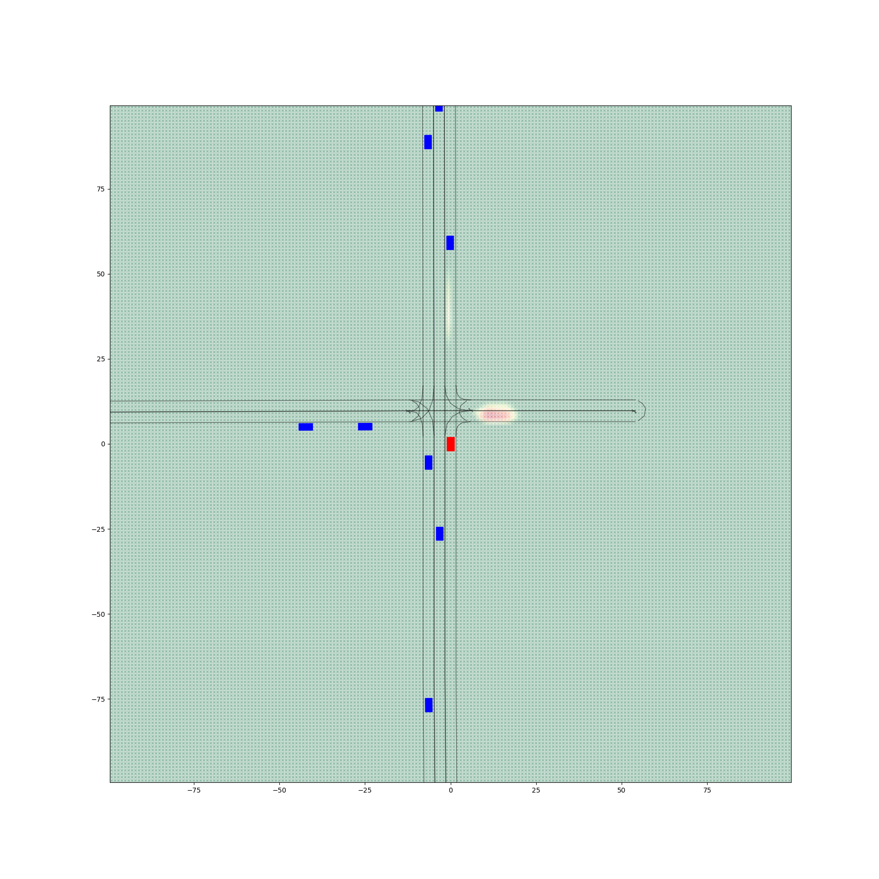
Figure 6 provides a comparative visualization of occupancy heatmaps generated by different encoder-decoder configurations, with a focus on the spatial accuracy and alignment of predicted probabilities with drivable areas. The figure demonstrates the progressive improvements achieved through the fine-tuning of the decoder.

Figures 6(a) and 6(d) illustrate the outputs from Encoder 0 and Encoder 1 paired with Decoder 0, respectively, before any fine-tuning. Despite producing visually realistic heatmaps, these configurations exhibit significant probabilities in non-drivable regions, with 4.79% of total occupancy values lying outside drivable areas for Encoder 0 + Decoder 0 and 5.18% for Encoder 1 + Decoder 0. These results highlight a critical limitation of the initial decoder: its inability to confine occupancy predictions to spatially relevant regions, undermining its practical utility.

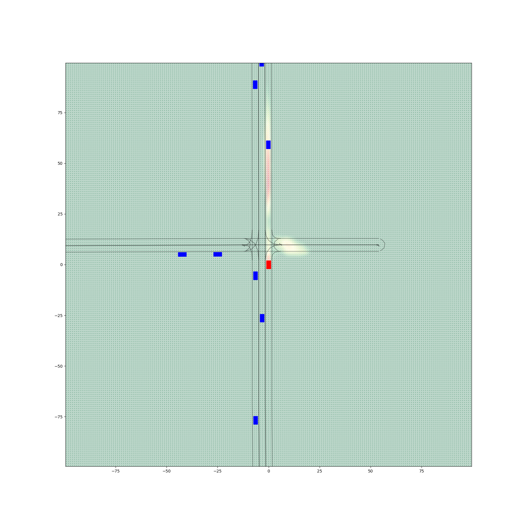
The second column, represented by figures 6(b) and 6(e), shows the results after fine-tuning the decoder using a filtered dataset to create Decoder 1. This refinement excluded the non-vehicle samples moving on pedestrian and bicycle lanes from the fine-tuning process. Consequently, both configurations exhibit a marked reduction in non-drivable area probabilities. Specifically, Encoder 0 + Decoder 1 reduces this proportion to 0.22%, while Encoder 1 + Decoder 1 achieves 0.55%. Although the predictions are still imperfect, the substantial improvement indicates the effectiveness of data filtering in enhancing spatial alignment.

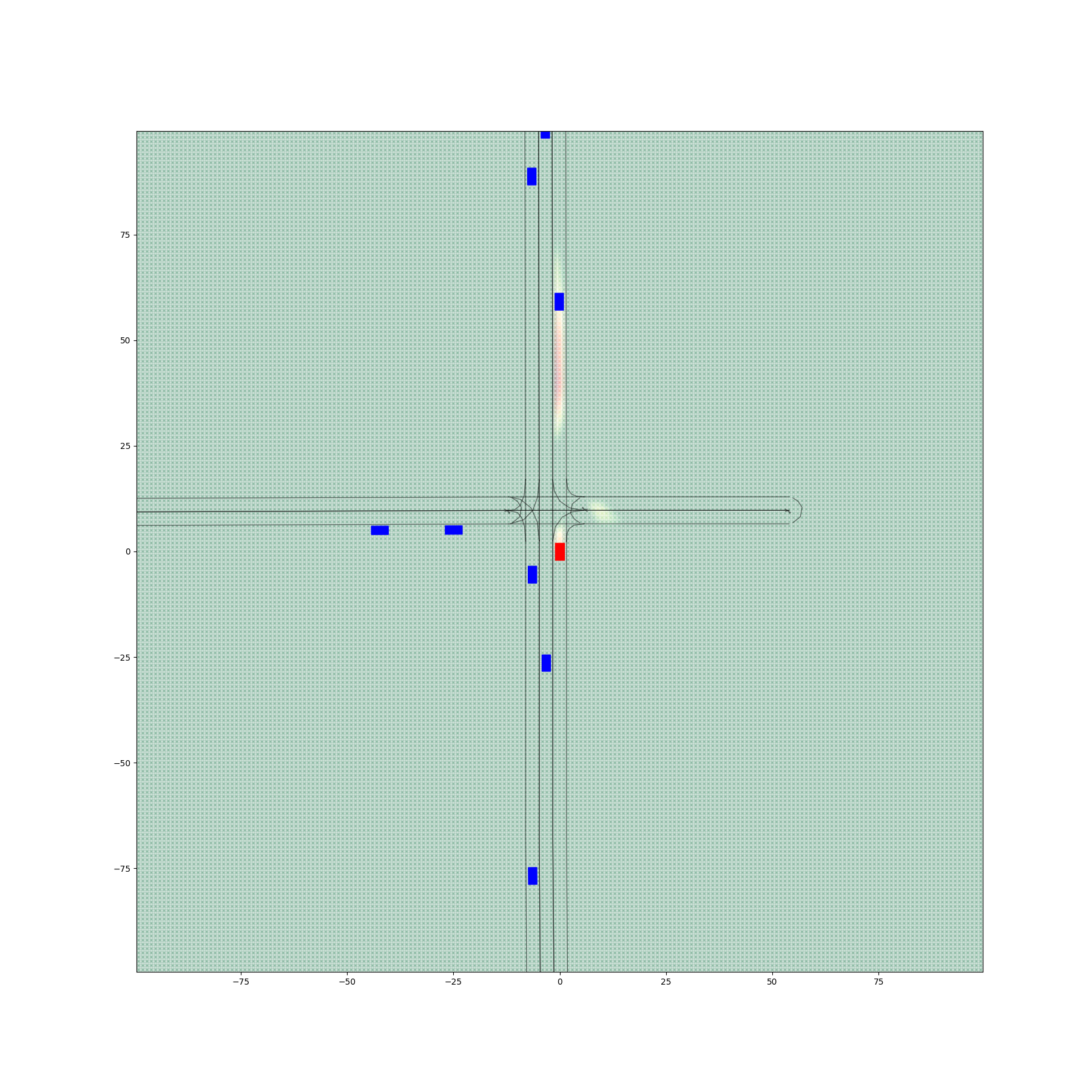
The third column, figures 6(c) and 6(f), presents the results from configurations using Decoder 2, which was fine-tuned with both the filtered dataset and a drivable area penalty term incorporated into the loss function. This penalty explicitly discourages high occupancy probabilities outside drivable areas, leading to a further refinement of predictions. Encoder 0 + Decoder 2 reduces the proportion of non-drivable predictions to 0.025%, while Encoder 1 + Decoder 2 achieves 0.066%. These configurations exhibit the most accurate spatial alignment, with predictions closely confined to drivable areas.

The analysis reveals two key findings: 1. Fine-tuning the decoder with a filtered dataset and penalty constraints significantly improves the spatial accuracy of occupancy heatmaps, reducing erroneous predictions in non-drivable regions. 2. Encoder 1, trained on a combination of Argoverse and SUMO data, consistently outperforms Encoder 0 in all configurations, demonstrating its generalizability to diverse traffic scenarios.

The combination of Encoder 1 and Decoder 2 emerges as the optimal configuration, achieving the highest fidelity in spatial alignment and practical applicability. These results underscore the importance of modular fine-tuning and tailored loss functions in enhancing the performance of probabilistic occupancy prediction frameworks for autonomous vehicles.

Figures 8, 9, 10, 11, 12, 13 provided in the Appendix, illustrate the detailed comparisons between various encoder-decoder configurations. Each figure represents a distinct traffic scenario, such as non-traditional intersections, left turns, and lane-changing maneuvers, to evaluate the spatial alignment and prediction accuracy of the proposed framework. The comparisons highlight the progression of improvements achieved through fine-tuning decoder components and demonstrate the robustness in confining occupancy predictions to drivable regions. Notably, the fine-tuned configurations consistently exhibit lower probabilities of non-drivable area predictions across diverse scenarios, underscoring the efficacy of the proposed modular training approach.

4 Discussion

This paper presents a modular framework for uncertainty-aware trajectory prediction in autonomous vehicles, addressing key challenges in ensuring safety and operational efficiency in dynamic traffic environments.

Modular Architecture and Benefits

The proposed modular architecture decouples encoder and decoder training, enabling flexibility to adapt to different traffic scenarios. Environment- or traffic participant-specific decoders, such as those for pedestrians, bicyclists, and vehicles, or for use in highway versus urban driving, can be trained independently, avoiding the inefficiency of retraining entire models. This design also supports integration of additional data, like high-definition maps, enhancing adaptability. This also enables new data, characterizing new AV operating location or weather environments for example, to be quickly and efficiently incorporated as that data is collected.

Heatmap Representation and Safety

Heatmaps provide probabilistic views of future vehicle positions, capturing uncertainties and enabling robust safety-critical decisions. They help autonomous vehicles anticipate collisions and high-risk scenarios by allowing AVs to efficiently detect those vehicle interactions without requiring extensive sampling of a large number of trajectories. This is especially significant when trying to anticipate potential collisions arising from low-probability vehicle trajectories. The improved awareness of potential risks ensures improved predictions with actionable decisions like lane changes and obstacle avoidance.

While the proposed modular framework demonstrates advancements in uncertainty-aware trajectory prediction, several avenues for future work remain. First, integrating richer contextual information, such as high-definition maps and dynamic environmental data, could further enhance prediction accuracy and adaptability. Additionally, exploring alternative training strategies, such as reinforcement learning, may improve the robustness of the model in highly interactive traffic scenarios. Future efforts will also focus on extending the framework to multi-agent prediction tasks, capturing complex interactions among vehicles and vulnerable road users. Finally, real-world deployment and validation in diverse environments will be critical to ensuring the scalability and reliability of the proposed approach in practical autonomous driving systems.

References

- [1] Jonathan W Lee, Han Wang, Kathy Jang, Amaury Hayat, Matthew Bunting, Arwa Alanqary, William Barbour, Zhe Fu, Xiaoqian Gong, George Gunter, et al. Traffic control via connected and automated vehicles: An open-road field experiment with 100 cavs. IEEE Control System Magazine, arXiv preprint arXiv:2402.17043, 2024.
- [2] Han Wang, Zhe Fu, Jonathan Lee, Hossein Nick Zinat Matin, Arwa Alanqary, Daniel Urieli, Sharon Hornstein, Abdul Rahman Kreidieh, Raphael Chekroun, William Barbour, et al. Hierarchical speed planner for automated vehicles: A framework for lagrangian variable speed limit in mixed autonomy traffic. arXiv preprint arXiv:2402.16993, 2024.
- [3] Han Wang, H Nick Zinat Matin, and Maria Laura Delle Monache. Reinforcement learning-based adaptive speed controllers in mixed autonomy condition. In 2024 European Control Conference (ECC), pages 1869–1874. IEEE, 2024.
- [4] Henggang Cui, Vladan Radosavljevic, Fang-Chieh Chou, Tsung-Han Lin, Thi Nguyen-Tu Nguyen, Tzu-Kuo Huang, Jeff Schneider, and Nemanja Djuric. Multimodal trajectory predictions for autonomous driving using deep convolutional networks. In Proceedings of the IEEE/CVF Conference on Computer Vision and Pattern Recognition, pages 14424–14432, 2019.
- [5] Yuning Chai, Benjamin Sapp, Mayank Bansal, and Dragomir Anguelov. Multipath: Multiple probabilistic anchor trajectory hypotheses for behavior prediction. In Conference on Robot Learning, pages 86–99. PMLR, 2019.
- [6] Xinshuo Weng, Boris Ivanovic, Yan Wang, Yue Wang, and Marco Pavone. Para-drive: Parallelized architecture for real-time autonomous driving. In Proceedings of the IEEE/CVF Conference on Computer Vision and Pattern Recognition, pages 15449–15458, 2024.
- [7] Marion Neumeier, Michael Botsch, Andreas Tollkühn, and Thomas Berberich. Variational autoencoder-based vehicle trajectory prediction with an interpretable latent space. In 2021 IEEE International Intelligent Transportation Systems Conference (ITSC), pages 820–827. IEEE, 2021.
- [8] Boris Ivanovic and Marco Pavone. Multimodal future trajectory predictions using conditional variational autoencoders. In 2020 IEEE International Conference on Robotics and Automation (ICRA), pages 2774–2781. IEEE, 2020.
- [9] Julian Wiederer, Julian Schmidt, Ulrich Kressel, Klaus Dietmayer, and Vasileios Belagiannis. Joint out-of-distribution detection and uncertainty estimation for trajectory prediction. In 2023 IEEE/RSJ International Conference on Intelligent Robots and Systems (IROS), pages 5487–5494. IEEE, 2023.
- [10] Juanwu Lu, Can Cui, Yunsheng Ma, Aniket Bera, and Ziran Wang. Quantifying uncertainty in motion prediction with variational Bayesian mixture. In Proceedings of the IEEE/CVF Conference on Computer Vision and Pattern Recognition, pages 15428–15437, 2024.
- [11] Tim Salzmann, Boris Ivanovic, Punarjay Chakravarty, and Marco Pavone. Trajectron++: Dynamically-feasible trajectory forecasting with heterogeneous data. In Computer Vision–ECCV 2020: 16th European Conference, Glasgow, UK, August 23–28, 2020, Proceedings, Part XVIII 16, pages 683–700. Springer, 2020.
- [12] Amir Rasouli. Deep learning for vision-based prediction: A survey. arXiv preprint arXiv:2007.00095, 2020.
- [13] Han Wang, Haochen Wu, Juanwu Lu, Fang Tang, and Maria Laura Delle Monache. Communication optimization for multi-agent reinforcement learning-based traffic control system with explainable protocol. In 2023 IEEE 26th International Conference on Intelligent Transportation Systems (ITSC), pages 6068–6073. IEEE, 2023.
- [14] Bernard Lange, Ekim Yurtsever, Seokcheon Yoon, and Mykel J Kochenderfer. Self-supervised multi-future occupancy forecasting for autonomous driving. arXiv preprint arXiv:2407.21126, 2023.
- [15] Jiazhi Yang, Shenyuan Gao, Yihang Qiu, Li Chen, Tianyu Li, Bo Dai, Kashyap Chitta, Penghao Wu, Jia Zeng, Ping Luo, et al. Generalized predictive model for autonomous driving. In Proceedings of the IEEE/CVF Conference on Computer Vision and Pattern Recognition, pages 14662–14672, 2024.
- [16] Eivind Meyer, Lars Frederik Peiss, and Matthias Althoff. Deep occupancy-predictive representations for autonomous driving. arXiv preprint arXiv:2303.04218, 2023.
- [17] Benjamin Wilson, William Qi, Tanmay Agarwal, John Lambert, Jagjeet Singh, Siddhesh Khandelwal, Bowen Pan, Ratnesh Kumar, Andrew Hartnett, Jhony Kaesemodel Pontes, Deva Ramanan, Peter Carr, and James Hays. Argoverse 2: Next generation datasets for self-driving perception and forecasting. In Proceedings of the Neural Information Processing Systems Track on Datasets and Benchmarks (NeurIPS Datasets and Benchmarks 2021), 2021.